Men’s Doubles Results

This is part of a series of reference posts that lay out what historical data is available at TennisAbstract.com. I recently did a similar post about pre-Open era men’s singles data. I’ll try to keep this post updated as the site expands.

Amateur-era doubles data–even doubles results from early in the Open era–is thin on the ground. I’m trying, slowly, to change that.

The TennisAbstract.com site now contains over 1,300 men’s doubles results from 1957 to 1967, the last eleven years of the amateur era. That includes:

  • Grand slam finals
  • All Davis Cup doubles rubbers
  • Doubles matches from professional tournaments and barnstorming stops. This varies enormously from year to year, in part because the pro tours sometimes played doubles every night, and sometimes they rarely did. At the extremes, I have 83 pro doubles matches from 1958 and only one from 1961. Reporting of these matches was extremely inconsistent at the time.
  • Doubles finals from all amateur tournaments where at least one member of the Tennis 128 competed–assuming I could find it. This amounts to roughly 60 finals per year, spanning most of the circuit’s most notable events.

Note my focus on finals. Eventually, I may expand on that, especially for grand slams. But collecting doubles results is extremely slow going, and contemporary coverage was much spottier than for singles. There’s nothing quite so disheartening as trying to add a match to the database when the losing side is listed only as “Smith/Smith.” Or worse: “Smith/partner.”

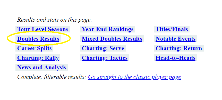
On any player page, you can find doubles results–assuming the player has some–by scrolling down, or by clicking here:

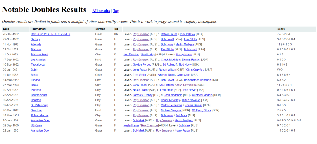
Here’s what you’ll see, at least if you’re on Rod Laver’s page:

Rocket was pretty good at doubles, too.

This “notable” table is limited to 20 matches. For most players, that’s all I have at this point. If I have more, the “notable” table lists a combination of slam finals and the most recent matches.

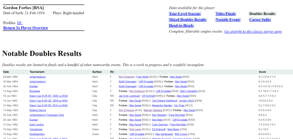
If there is an “All results” link above the table–as there is for Laver–that means I have more than 20 matches, and you can click through to get the full list. Here, for instance, is Gordon Forbes:

By the time he retired, the man had a lot to write about.

Eventually, these pages will be filterable, like the singles results. For now, it’s just a reverse-chronological list.

Next up, I hope to add men’s doubles from the 1968 season, as well as a few more seasons from the beginning of the Open era. Then I’ll go back to 1956 and add more amateur-era seasons.

* * *

Subscribe to the blog to receive each new post by email:


Pre-Open Era Men’s Singles Results

This is the first in a series of reference posts that aim to describe what historical data is available at TennisAbstract.com. My goal is to keep these updated as the site continues to expand.

TennisAbstract.com now contains approximately 37,000 men’s singles results from the years 1957-67, the decade-plus that preceded the Open Era. The site has a reasonably complete set of pro results from 1968 to present, though I occasionally plug gaps and make corrections there as well.

Remarkably, 37,000 matches is nowhere near a complete representation of eleven years of amateur-era tennis.

Here’s what you can now find on the site for the years 1957-67:

  • Complete grand slam singles results
  • Complete Davis Cup singles results
  • Every professional match I’ve been able to find, including matches from pro tours, which often featured just one or two singles matches per stop
  • Every singles match from any tournament where a member of the Tennis 128 competed (not just matches involving Tennis 128ers).

The last category is quirky: It means that I now have results for some minor tournaments, like the Romanian National Championships when Ilie Năstase entered as a young man, or some regional collegiate events where Arthur Ashe or Stan Smith competed. It also means I lack some significant events–for instance, some editions of the U.S. Indoors or Bournemouth–if no 128ers happened to enter that year.

Despite the odd way I’ve drawn the line, the result is a pretty good representation of each season, one that includes most of the notable events. The decision also means that as I work backwards, I’ll complete–insofar as it is possible–the careers of the most historically significant players.

My goal is to make one pass back to 1920 or so before going through each year again, at which point I’ll shoot for a much more thorough level of coverage. Even this “limited” approach means adding more than 3,000 matches per season. That’s enough for the moment, at least if I hope ever to finish.

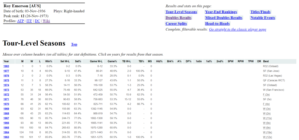
You can browse all this data the same way you view results for current players. For instance, here are the yearly summaries for Roy Emerson:

Yeah, that peak rank of 12 doesn’t really tell the story. Amateur-era expert rankings are also on my (breathtakingly long) to-do list.

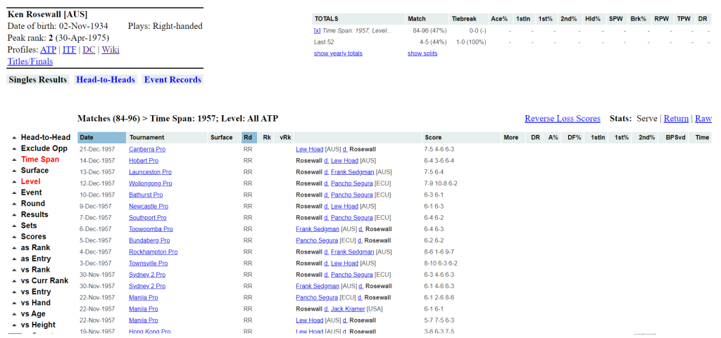
And here are some match-by-match results for Ken Rosewall at the end of his first pro season, in 1957:

#2 isn’t quite right for Muscles, either.

Next, I plan to fill in some gaps in the first few years of the Open era, then jump back to 1956 and work backwards from there.

* * *

Subscribe to the blog to receive each new post by email:


The Tournament Simulation Reference

Italian translation at settesei.it

Among the more popular features of Heavy Topspin are my tournament forecasts, based on draw simulations.  It’s about time that I summarize how these work.

Monte Carlo simulations

To generate tournament predictions, we first need a way to predict the outcome of individual matches.  For that, I use jrank, which I’ve written about elsewhere.  With numerical estimates of a player’s skill–not unlike ATP ranking points–we can calculate the probability that each player wins the match.

Once those matchup probabilities are calculated, it’s a matter of “playing” the tournament thousands upon thousands of times.  Here, computers come in awfully handy.

My code (a version of which is publicly available) uses a random-number generator (RNG) to determine the winner of each match.  For instance, at the top of the Rogers Cup draw this week, Novak Djokovic gets a bye, after which he’ll play the winner of Bernard Tomic‘s match with Michael Berrer.  My numbers give Tomic a 64% chance of beating Berrer.  To “play” that match in a simulated tournament, the RNG spits out a number between 0 and 1.  If the result is below .64, Tomic is the winner; if not, Berrer wins.

The winner advances to “play” Djokovic.  The code determines Djokovic’s probability of beating whoever advances to play him, then generates a new random number to pick the winner.  Repeat the process 47 times–one for each match–and you’ve simulated the entire tournament.

Each simulation, then, gives us a set of results.  Perhaps Tomic reaches the second round, losing to Djokovic, who then loses in the quarters to Juan Martin Del Potro, who goes on to win the tournament.   That’s one possibility–and it’s more likely than many alternatives–but it doesn’t tell the whole story.

That’s why we do it thousands (or even millions) of times.  Over that many simulations, Delpo occasionally wins, but somewhat more often, Djokovic wins that quarterfinal showdown.  Tomic usually reaches the second round, but sometimes it’s Berrer into the second round.  All of these “usually’s” and “sometimes’s” are converted into percentages based on just how often they occur.

Probability adjustments

For any given pair of players, we don’t always expect the same outcome.  Pablo Andujar is almost always the underdog on hardcourts, but we expect him to beat most mid-packers on clay.  Players perform (a bit) better in their home country.  Qualifiers do worse than equivalent players who didn’t have to qualify.

Thus, if we take last week’s Washington field and transplant it to the clay courts of Vina Del Mar, the numbers would change a great deal.  Americans and hard-court specialists would see their chances decrease, while Chileans and clay-courters would see theirs increase–just as conventional wisdom suggests would happen.

Simulation variations: Draw-independence

Some of the more interesting results come from messing around with the draw.  Every time a field is arranged into a bracket, there are winners and losers.  Whoever is drawn to face the top seed in the first round (or second, as Berrer and Tomic can attest) is probably unlucky, while somewhere else in the draw, a couple of lucky qualifiers get to play each other for a spot in the second round.

That’s one of the reasons I sometimes run draw-independent simulations (DIS).  If we want to know how much the draw helped or hurt a player, we need to know how successful he was likely to be before he was placed in the draw.  (DISs are also handy if you know the likely field, but the draw isn’t yet set.)

To run a draw-independent sim, we have to start one step earlier.  Instead of taking the draw as a given, we take the field as a given, including the seedings if we know them.  Then we use the same logic as tournament officials will use in constructing the draw.  The #1 seed goes at the top, #2 at the bottom.  #3 and #4 are randomly placed in the remaining quarters.  #5 through #8 are randomly placed in the remaining eighths, and so on.

(Update: I’ve published a python function, reseeder(), which generates random draws for any combination of number of seeds and field size that occurs on the ATP tour.)

Simulation variations: Seed-independence

We can take this even further to measure the beneficial effect of seeding.  Most of the time we take seeding for granted–we want the top two players in the world to clash only in the final, and so on.  But it can have a serious effect on a player’s chances of winning a tournament.  In Toronto this week, the top 16 seeds (along with, in all likelihood, a very lucky loser or two) get a bye straight into the second round.  That helps!

Even when there are no byes, seedings guarantee relatively easy matches for the first couple of rounds.  That may not make a huge difference for someone like Djokovic–he’ll cruise whether he draws a seeded Florian Mayer or an unseeded Jeremy Chardy.  But if you are Mayer, consider the benefits.  You’re barely better than some unseeded players, but you’re guaranteed to miss the big guns until the third round.

This is why we talk so much about getting into the top 32 in time for slams.  When the big points and big money are on the line, you want those easy opening matches even more than usual.  There isn’t much separating Kevin Anderson from Sam Querrey, but if the US Open draw were held today, Anderson would get a seed and Querrey wouldn’t.  Guess who we’d be more likely to see in the third round!

To run a seed-independent simulation: Instead of generating a logical draw, as we do with a DIS, generate a random draw, in which anyone can face anyone in the first round.

Measuring variations

If we compare forecasts based on the actual draw to draw-independent or seed-independent forecasts, we want to quantify the difference.  To do so, I’ve used two metrics: Expected Ranking Points (ERP) and Expected Prize Money (EPM).

Both reduce an entire tournament’s worth of forecasts to one number per player.  If Djokovic has a 30% chance of winning this week in Toronto, that’s the probability he’ll take home 1,000 points.  If those were the only points on offer, his ERP would be 30% of 1,000, or 300.

Of course, if Djokovic loses, he’ll still get some points.  To come up with his overall ERP, we consider his probability of losing the finals and the number of points awarded to the losing finalist, his probability of losing in the semis and the number of points awarded to semifinalists, and so on.  To calculate EPM, we use the same process, but with–you guessed it–prize money instead of ranking points.

Both numbers allow to see how much the draw helps or hurts a player.  For instance, before the French Open, I calculated that Richard Gasquet‘s EPM rose by approximately 25% thanks to a very lucky draw.

These numbers also help us analyze a player’s scheduling choices.  The very strong Olympics field and the much weaker Washington field last week created an odd situation: Lesser players were able to rack up far more points than their more accomplished colleagues. Even before the tournament, we could use the ERP/EPM approach to see that Mardy Fish could expect 177 points in Washington while the far superior David Ferrer could expect only 159 in London.

If you’ve read this far, you will probably enjoy the newest feature on TennisAbstract.com–live-ish forecast updates for all ATP events.  Find links on the TA.com homepage, or click straight to the Rogers Cup page.
The Official JRank Reference

Italian translation at settesei.it

At HeavyTopspin, I frequently post references to “my rankings” which power my tournament projections.  (For instance, 2012 French Open men and women.)  My system is unofficially called “JRank”–in other words, it needs a new name.    The rankings it generates are superior to the ATP (and presumably WTA) rankings in the sense that they better predict the outcome of tour- and challenger-level matches.

The algorithm is complex but the ideas behind it are not.  The fundamental difference between JRank and the ATP system is how it values individual matches.

The ATP system awards points based on tournament and round.  (A first round win at Wimbledon is worth more than a first round win at Halle; a third round win at Roland Garros is worth more than a second round win.)  JRank, by contrast, awards points based on opponent and recency.  In my system, a win against Rafael Nadal is worth much more than a defeat of Igor Kunitsyn, even if both take place in the same round at the same tournament.  And a defeat of Kunitsyn is worth more if it took place last week than if it took place eight months ago.  A recent win tells you more about a player’s current ability level than an older one does.

The advantage of giving recent matches more weight is that it allows us to take into account matches more than one year old, without the veteran-favoring disadvantages of Nadal’s two-year plan.  JRank uses all matches from the last two years, but a match one year ago is worth only half as much as a match last week, while a match two years ago is worth only a quarter as much.  That way, we get the benefits of that much more data, but without unduly favoring vets.  There is the added benefit that JRank is “smoother” from week to week–none of the bizarre effects of a tournament “falling off” from last year–as if a player’s results 51 weeks ago are 100% more relevant than his results 54 weeks ago!

JRank’s value is even greater because it generates separate rankings for clay and hard surfaces.  Everyone knows that surface matters, but the ATP ranking system ignores it completely.  If you want to know who should be favored at the French, it seems silly to weight Bercy as heavily as Monte Carlo.  JRank gives more weight to a player’s clay record for his clay ranking, and so on.  Even further, beating a clay court specialist is worth more on clay than it is on a hard court.

Creating projections

Armed with rankings, it’s a few small steps to generating a forecast for any tournament.  For each match, the projection is based almost entirely on the rankings of the two players.  (The formula is a slightly more complicated version of A divided by A+B, where A is one player’s ranking point and B is the other’s.  It works–approximately–with ATP ranking points as well.)

There are a few tweaks, though.  First, my research has indicated that qualifiers, lucky losers, and wild cards all perform slightly below expectations.  It is unclear why, though with qualifiers I suspect it is due to fatigue–while their opponents rested, they played two or three tough matches to qualify.

Second, I’ve established that there is a slight home court advantage.  When surface is accounted for, home court advantage is minimal, but it is still there–the “home” player performs about 2% better than expected.  Perhaps it’s referee bias, home cooking, fan support, or some combination of the above.

A frequent suggestion is to incorporate head-to-head records into match projections.  It’s a tempting idea–so tempting that I’ve tried it.  However, it doesn’t seem to make much difference, at least for any broad cross-section of matches.  (Perhaps when a pair of players have, say, 10 or more head-to-head matches in the books, stronger patterns emerge.)  For the most part, it seems that if a ranking system represents a good approximation of each player’s ability level, head-to-head results are superfluous.

There may be other variables worth looking at, including the importance of the tournament, the player’s fatigue level or recent injury history, or each player’s experience at a particular event.  For now, those are among the influences I haven’t even tested.